SAR example
Contents
SAR example#
Let’s use EOReader with SAR data.
Warning: SAR data is processed with SNAP, so be sure to have it installed and that GPT is in your path.
Imports#
import os
import logging
import matplotlib.pyplot as plt

# EOReader
from eoreader.reader import Reader
from eoreader.bands import *
from eoreader.env_vars import DEM_PATH
Create logger#
# Create logger

logger = logging.getLogger("eoreader")
logger.setLevel(logging.INFO)

# create console handler and set level to debug
ch = logging.StreamHandler()
ch.setLevel(logging.INFO)

# create formatter
formatter = logging.Formatter('%(message)s')

# add formatter to ch
ch.setFormatter(formatter)

# add ch to logger
logger.addHandler(ch)
Open the COSMO-SkyMed product#
Please be aware that:
EOReader will orthorectify your SAR data to get UTM tiles.
complex data is not handled as is, EOReader will convert them to ground range.
# First of all, we need some VHR data, let's use some COSMO-SkyMed data
path = os.path.join("/home", "data", "DATA", "PRODS", "COSMO", "1st_GEN", "1001512-735097")

# Open your product
prod = Reader().open(path, remove_tmp=True)
prod
EOReader CskProduct
Attributes:
	condensed_name: 20201008T224018_CSK_HI_DGM
	name: CSKS4_DGM_B_HI_09_HH_RA_FF_20201008224018_20201008224025
	path: /home/data/DATA/PRODS/COSMO/1st_GEN/1001512-735097
	platform: COSMO-SkyMed
	sensor type: SAR
	product type: DGM
	default resolution: 5.0
	acquisition datetime: 2020-10-08T22:40:18.446381
	band mapping:
		VV: VV
		VV_DSPK: VV_DSPK
		HH: HH
		HH_DSPK: HH_DSPK
		VH: VH
		VH_DSPK: VH_DSPK
		HV: HV
		HV_DSPK: HV_DSPK
		RH: RH
		RH_DSPK: RH_DSPK
		RV: RV
		RV_DSPK: RV_DSPK
	needs extraction: True
	orbit direction:ASCENDING
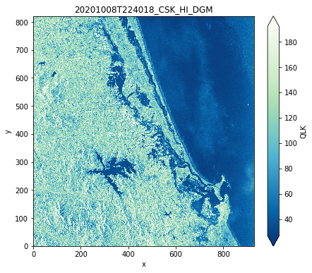
# Plot the quicklook
prod.plot()
# Print some data
print(f"Acquisition datetime: {prod.datetime}")
print(f"Condensed name: {prod.condensed_name}")
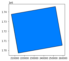
# Open here some more interesting geographical data: extent and footprint
extent = prod.extent()
footprint = prod.footprint()
base = extent.plot(color='cyan', edgecolor='black')
footprint.plot(ax=base, color='blue', edgecolor='black', alpha=0.5)
Acquisition datetime: 2020-10-08 22:40:18.446381
Condensed name: 20201008T224018_CSK_HI_DGM
Executing processing graph
....10%....20%....30%....40%....50%....60%....70%....80%....90% done.
<AxesSubplot:>
For SAR data, the footprint needs the orthorectified data !
For that, SNAP uses its own DEM, but you can change it when positionning the EOREADER_SNAP_DEM_NAME environment variable.
Available DEMs are:
ACE2_5MinACE30ASTER 1sec GDEMCopernicus 30m Global DEM(buggy for now, do not use it)Copernicus 90m Global DEM(buggy for now, do not use it)GETASSE30(by default)SRTM 1Sec HGTSRTM 3SecExternal DEM
Warning:
If External DEM is set, you must specify the DEM you want by positioning the EOREADER_DEM_PATH to a DEM that can be read by SNAP.
Load bands#
# Set the DEM
os.environ[DEM_PATH] = os.path.join("/home", "data", "DS2", "BASES_DE_DONNEES", "GLOBAL", "COPDEM_30m", "COPDEM_30m.vrt")

# Select some bands you wish to load without knowing if they exist
bands = [VV, HH, VV_DSPK, HH_DSPK, HILLSHADE, SLOPE]

# Only keep those selected
ok_bands = [band for band in bands if prod.has_band(band)]

# This product does not have VV band and HILLSHADE band cannot be computed from SAR band
print(to_str(ok_bands))
['HH', 'HH_DSPK', 'SLOPE']
# Load those bands as a dict of xarray.DataArray, with a 20m resolution
band_dict = prod.load(ok_bands, resolution=20.)
band_dict[HH]
Executing processing graph
first_line_time metadata value is null
last_line_time metadata value is null
...10%...21%...32%...43%...54%...65%...76%...87%. done.
<xarray.DataArray 'HH' (band: 1, y: 2474, x: 2689)>
array([[[nan, nan, nan, ..., nan, nan, nan],
        [nan, nan, nan, ..., nan, nan, nan],
        [nan, nan, nan, ..., nan, nan, nan],
        ...,
        [nan, nan, nan, ..., nan, nan, nan],
        [nan, nan, nan, ..., nan, nan, nan],
        [nan, nan, nan, ..., nan, nan, nan]]], dtype=float32)
Coordinates:
  * x            (x) float64 2.058e+05 2.059e+05 ... 2.596e+05 2.596e+05
  * y            (y) float64 1.746e+06 1.746e+06 ... 1.697e+06 1.697e+06
  * band         (band) int64 1
    spatial_ref  int64 0
Attributes:
    scale_factor:      1.0
    add_offset:        0.0
    long_name:         HH
    sensor:            COSMO-SkyMed
    sensor_id:         CSK
    product_path:      /home/data/DATA/PRODS/COSMO/1st_GEN/1001512-735097
    product_name:      CSKS4_DGM_B_HI_09_HH_RA_FF_20201008224018_20201008224025
    product_filename:  1001512-735097
    product_type:      DGM
    acquisition_date:  20201008T224018
    condensed_name:    20201008T224018_CSK_HI_DGM
orbit_direction: ASCENDINGThis can lead the Terrain Correction step to create large nodata area when projecting on a DEM.
If it happens, you can set the keyword SAR_INTERP_NA to True when loading or stacking SAR data to fill these area with interpolated data.
from eoreader.keywords import SAR_INTERP_NA
band_dict = prod.load(
    ok_bands,
    resolution=20.,
    **{SAR_INTERP_NA: True}
)
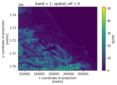
# Plot a subsampled version
band_dict[SLOPE][:, ::10, ::10].plot()
<matplotlib.collections.QuadMesh at 0x7efbe57c1910>
Stack some data#
# You can also stack those bands
stack = prod.stack(ok_bands)
stack
<xarray.DataArray 'HH_HH_DSPK_SLOPE' (z: 3, y: 9897, x: 10755)>
array([[[        nan,         nan,         nan, ...,         nan,
                 nan,         nan],
        [        nan,         nan,         nan, ...,         nan,
                 nan,         nan],
        [        nan,         nan,         nan, ...,         nan,
                 nan,         nan],
        ...,
        [        nan,         nan,         nan, ...,         nan,
                 nan,         nan],
        [        nan,         nan,         nan, ...,         nan,
                 nan,         nan],
        [        nan,         nan,         nan, ...,         nan,
                 nan,         nan]],

       [[        nan,         nan,         nan, ...,         nan,
                 nan,         nan],
        [        nan,         nan,         nan, ...,         nan,
                 nan,         nan],
        [        nan,         nan,         nan, ...,         nan,
                 nan,         nan],
...
        [        nan,         nan,         nan, ...,         nan,
                 nan,         nan],
        [        nan,         nan,         nan, ...,         nan,
                 nan,         nan],
        [        nan,         nan,         nan, ...,         nan,
                 nan,         nan]],

       [[ 0.4255329 ,  0.4255329 ,  0.4255329 , ...,  0.        ,
          0.        ,  0.        ],
        [ 0.4255329 ,  0.4255329 ,  0.4255329 , ...,  0.        ,
          0.        ,  0.        ],
        [ 0.4255329 ,  0.4255329 ,  0.4255329 , ...,  0.        ,
          0.        ,  0.        ],
        ...,
        [16.66219   , 16.66219   , 16.66219   , ...,  0.0870695 ,
          0.0870695 ,  0.0870695 ],
        [16.66219   , 16.66219   , 16.66219   , ...,  0.0870695 ,
          0.0870695 ,  0.0870695 ],
        [17.018255  , 17.018255  , 17.018255  , ...,  0.08737368,
          0.08737368,  0.08737368]]], dtype=float32)
Coordinates:
    spatial_ref  int64 0
  * x            (x) float64 2.058e+05 2.058e+05 ... 2.596e+05 2.596e+05
  * y            (y) float64 1.746e+06 1.746e+06 ... 1.697e+06 1.697e+06
  * z            (z) MultiIndex
  - variable     (z) object 'HH' 'HH_DSPK' 'SLOPE'
  - band         (z) int64 1 1 1
Attributes:
    long_name:         HH HH_DSPK SLOPE
    sensor:            COSMO-SkyMed
    sensor_id:         CSK
    product_path:      /home/data/DATA/PRODS/COSMO/1st_GEN/1001512-735097
    product_name:      CSKS4_DGM_B_HI_09_HH_RA_FF_20201008224018_20201008224025
    product_filename:  1001512-735097
    product_type:      DGM
    acquisition_date:  20201008T224018
    condensed_name:    20201008T224018_CSK_HI_DGM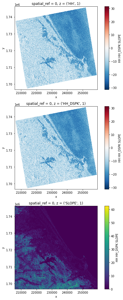
orbit_direction: ASCENDING# Plot a subsampled version
nrows = len(stack)
fig, axes = plt.subplots(nrows=nrows, figsize=(3 * nrows, 6 * nrows), subplot_kw={"box_aspect": 1})
for i in range(nrows):
stack[i, ::10, ::10].plot(x="x", y="y", ax=axes[i])