Exogenous data management

Any exogenous data can be loaded in EOReader. The data will be collocated onto the product grid.

Here is the way.

# Imports
import os

import matplotlib.pyplot as plt

from rasterio.enums import Resampling

from sertit import AnyPath
from eoreader.bands import to_str
from eoreader.reader import Reader
from eoreader.keywords import EXO_KW

# Create logger
import logging
from sertit import logs

logger = logging.getLogger("eoreader")
logs.init_logger(logger)

# Open the product
exo_folder = AnyPath("/home/prods/EXOGENOUS")
path = exo_folder / "S2C_MSIL2A_20251017T111101_N0511_R137_T32VLM_20251017T151300.SAFE"
prod = Reader().open(path)
prod

eoreader.S2Product 'S2C_MSIL2A_20251017T111101_N0511_R137_T32VLM_20251017T151300'
Attributes:
	condensed_name: 20251017T111101_S2_T32VLM_L2A_151300
	path: /home/prods/EXOGENOUS/S2C_MSIL2A_20251017T111101_N0511_R137_T32VLM_20251017T151300.SAFE
	constellation: Sentinel-2
	sensor type: Optical
	product type: MSIL2A
	default pixel size: 10.0
	default resolution: 10.0
	acquisition datetime: 2025-10-17T11:11:01
	band mapping:
		COASTAL_AEROSOL: 01
		BLUE: 02
		GREEN: 03
		RED: 04
		VEGETATION_RED_EDGE_1: 05
		VEGETATION_RED_EDGE_2: 06
		VEGETATION_RED_EDGE_3: 07
		NIR: 08
		NARROW_NIR: 8A
		WATER_VAPOUR: 09
		SWIR_1: 11
		SWIR_2: 12
	needs extraction: False
	cloud cover: 2.722754
	tile name: T32VLM

# Exogenous data path
mosaic_s1 = exo_folder / "Sentinel-1_IW_mosaic_2025_M11_32VLM_0_0_VV.tif"
!gdalinfo $mosaic_s1

Driver: GTiff/GeoTIFF
Files: /home/prods/EXOGENOUS/Sentinel-1_IW_mosaic_2025_M11_32VLM_0_0_VV.tif
Size is 5004, 5004
Coordinate System is:
PROJCRS["WGS 84 / UTM zone 32N",
    BASEGEOGCRS["WGS 84",
        DATUM["World Geodetic System 1984",
            ELLIPSOID["WGS 84",6378137,298.257223563,
                LENGTHUNIT["metre",1]]],
        PRIMEM["Greenwich",0,
            ANGLEUNIT["degree",0.0174532925199433]],
        ID["EPSG",4326]],
    CONVERSION["UTM zone 32N",
        METHOD["Transverse Mercator",
            ID["EPSG",9807]],
        PARAMETER["Latitude of natural origin",0,
            ANGLEUNIT["degree",0.0174532925199433],
            ID["EPSG",8801]],
        PARAMETER["Longitude of natural origin",9,
            ANGLEUNIT["degree",0.0174532925199433],
            ID["EPSG",8802]],
        PARAMETER["Scale factor at natural origin",0.9996,
            SCALEUNIT["unity",1],
            ID["EPSG",8805]],
        PARAMETER["False easting",500000,
            LENGTHUNIT["metre",1],
            ID["EPSG",8806]],
        PARAMETER["False northing",0,
            LENGTHUNIT["metre",1],
            ID["EPSG",8807]]],
    CS[Cartesian,2],
        AXIS["(E)",east,
            ORDER[1],
            LENGTHUNIT["metre",1]],
        AXIS["(N)",north,
            ORDER[2],
            LENGTHUNIT["metre",1]],
    USAGE[
        SCOPE["Navigation and medium accuracy spatial referencing."],
        AREA["Between 6°E and 12°E, northern hemisphere between equator and 84°N, onshore and offshore. Algeria. Austria. Cameroon. Denmark. Equatorial Guinea. France. Gabon. Germany. Italy. Libya. Liechtenstein. Monaco. Netherlands. Niger. Nigeria. Norway. Sao Tome and Principe. Svalbard. Sweden. Switzerland. Tunisia. Vatican City State."],
        BBOX[0,6,84,12]],
    ID["EPSG",32632]]
Data axis to CRS axis mapping: 1,2
Origin = (300000.000000000000000,6700020.000000000000000)
Pixel Size = (20.000000000000000,-20.000000000000000)
Metadata:
  AREA_OR_POINT=Area
  TIFFTAG_RESOLUTIONUNIT=1 (unitless)
  TIFFTAG_XRESOLUTION=1
  TIFFTAG_YRESOLUTION=1
Image Structure Metadata:
  COMPRESSION=DEFLATE
  INTERLEAVE=BAND
  LAYOUT=COG
  PREDICTOR=3
Corner Coordinates:
Upper Left  (  300000.000, 6700020.000) (  5d22'14.30"E, 60d23'13.15"N)
Lower Left  (  300000.000, 6599940.000) (  5d28' 2.84"E, 59d29'24.32"N)
Upper Right (  400080.000, 6700020.000) (  7d11' 6.62"E, 60d25'26.75"N)
Lower Right (  400080.000, 6599940.000) (  7d14' 1.23"E, 59d31'33.20"N)
Center      (  350040.000, 6649980.000) (  6d18'51.24"E, 59d57'35.36"N)
Band 1 Block=256x256 Type=Float32, ColorInterp=Gray
  NoData Value=-32768
  Overviews: 2502x2502, 1251x1251, 626x626, 313x313

Then you may load specific layer from the EXO folder using the load or stack function.

To do this, you need to provide the EXO_KW. The expected value is a dictionnary containing the target name of the layer as key, and the path as sub-attribute.

In the case where the file provide as path is multi-layer, you must specify the bandnumber to load. Band indexes start at 1, if the band index does not exist it returns an array of nan, default: 1.

You can also change the resampling method to apply, by using resampler. Supported options any Resampling value from rasterio, such as nearest or bilinear.

# Load the bands
loaded_bands = prod.load(
    ['GREEN'],
    pixel_size=100.,
    **{
        EXO_KW: {'Sentinel-1_2025/11_mosaic': {'bandnumber' : 1, 'path' : mosaic_s1, 'resampler' : 'nearest'}},     
    }
)

# Display the xarray.Dataset
loaded_bands

2025-12-23 11:44:13,619 - [DEBUG] - Loading bands ['GREEN']
2025-12-23 11:44:13,642 - [DEBUG] - Read GREEN
2025-12-23 11:44:14,436 - [DEBUG] - Manage nodata for band GREEN
2025-12-23 11:44:14,639 - [DEBUG] - Converting GREEN to reflectance (if needed)
2025-12-23 11:44:14,701 - [DEBUG] - Clip the reflectance array to 0 as minimum value (in some cases, reflectance can have higher value than 1)
2025-12-23 11:44:25,332 - [INFO] - Loading exogenous bands
2025-12-23 11:44:25,332 - [DEBUG] - EXO data info: Sentinel-1_2025/11_mosaic ; {'bandnumber': 1, 'path': PosixPath('/home/prods/EXOGENOUS/Sentinel-1_IW_mosaic_2025_M11_32VLM_0_0_VV.tif'), 'resampler': 'nearest'}
2025-12-23 11:44:25,333 - [DEBUG] - Warping EXO for 20251017T111101_S2_T32VLM_L2A_151300
2025-12-23 11:44:25,334 - [DEBUG] - Using EXO: /home/prods/EXOGENOUS/Sentinel-1_IW_mosaic_2025_M11_32VLM_0_0_VV.tif

<xarray.Dataset> Size: 10MB
Dimensions:                    (x: 1098, y: 1098, band: 1)
Coordinates:
  * x                          (x) float64 9kB 3e+05 3.002e+05 ... 4.098e+05
  * y                          (y) float64 9kB 6.7e+06 6.7e+06 ... 6.59e+06
    spatial_ref                int64 8B 0
  * band                       (band) int64 8B 1
Data variables:
    SpectralBandNames.GREEN    (band, y, x) float32 5MB dask.array<chunksize=(1, 102, 102), meta=np.ndarray>
    Sentinel-1_2025/11_mosaic  (band, y, x) float32 5MB dask.array<chunksize=(1, 1024, 1024), meta=np.ndarray>
Attributes:
    long_name:         GREEN Sentinel-1_2025/11_mosaic
    constellation:     Sentinel-2
    constellation_id:  S2
    product_path:      /home/prods/EXOGENOUS/S2C_MSIL2A_20251017T111101_N0511...
    product_name:      S2C_MSIL2A_20251017T111101_N0511_R137_T32VLM_20251017T...
    product_filename:  S2C_MSIL2A_20251017T111101_N0511_R137_T32VLM_20251017T...
    instrument:        MSI
    product_type:      MSIL2A
    acquisition_date:  20251017T111101
    condensed_name:    20251017T111101_S2_T32VLM_L2A_151300
    orbit_direction:   DESCENDING
    cloud_cover:       2.722754

xarray.Dataset

• Dimensions:
  • x: 1098
  • y: 1098
  • band: 1
• Coordinates: (4)
  • x
    (x)
    float64
    3e+05 3.002e+05 ... 4.098e+05

    array([300050., 300150., 300250., ..., 409550., 409650., 409750.],
          shape=(1098,))

  • y
    (y)
    float64
    6.7e+06 6.7e+06 ... 6.59e+06

    array([6699970., 6699870., 6699770., ..., 6590470., 6590370., 6590270.],
          shape=(1098,))

  • spatial_ref
    ()
    int64
    0

    spatial_ref :

    PROJCS["WGS 84 / UTM zone 32N",GEOGCS["WGS 84",DATUM["WGS_1984",SPHEROID["WGS 84",6378137,298.257223563,AUTHORITY["EPSG","7030"]],AUTHORITY["EPSG","6326"]],PRIMEM["Greenwich",0,AUTHORITY["EPSG","8901"]],UNIT["degree",0.0174532925199433,AUTHORITY["EPSG","9122"]],AUTHORITY["EPSG","4326"]],PROJECTION["Transverse_Mercator"],PARAMETER["latitude_of_origin",0],PARAMETER["central_meridian",9],PARAMETER["scale_factor",0.9996],PARAMETER["false_easting",500000],PARAMETER["false_northing",0],UNIT["metre",1,AUTHORITY["EPSG","9001"]],AXIS["Easting",EAST],AXIS["Northing",NORTH],AUTHORITY["EPSG","32632"]]

    crs_wkt :

    PROJCS["WGS 84 / UTM zone 32N",GEOGCS["WGS 84",DATUM["WGS_1984",SPHEROID["WGS 84",6378137,298.257223563,AUTHORITY["EPSG","7030"]],AUTHORITY["EPSG","6326"]],PRIMEM["Greenwich",0,AUTHORITY["EPSG","8901"]],UNIT["degree",0.0174532925199433,AUTHORITY["EPSG","9122"]],AUTHORITY["EPSG","4326"]],PROJECTION["Transverse_Mercator"],PARAMETER["latitude_of_origin",0],PARAMETER["central_meridian",9],PARAMETER["scale_factor",0.9996],PARAMETER["false_easting",500000],PARAMETER["false_northing",0],UNIT["metre",1,AUTHORITY["EPSG","9001"]],AXIS["Easting",EAST],AXIS["Northing",NORTH],AUTHORITY["EPSG","32632"]]

    GeoTransform :

    300000.0 100.0 0.0 6700020.0 0.0 -100.0

    array(0)

  • band
    (band)
    int64
    1

    array([1])

• Data variables: (2)
  • SpectralBandNames.GREEN
    (band, y, x)
    float32
    dask.array<chunksize=(1, 102, 102), meta=np.ndarray>

    path :

    /tmp/tmpwdfn5qhp/tmp_20251017T111101_S2_T32VLM_L2A_151300/20251017T111101_S2_T32VLM_L2A_151300_GREEN_100m_nodata.tif

    long_name :

    GREEN

    constellation :

    Sentinel-2

    constellation_id :

    S2

    product_path :

    /home/prods/EXOGENOUS/S2C_MSIL2A_20251017T111101_N0511_R137_T32VLM_20251017T151300.SAFE

    product_name :

    S2C_MSIL2A_20251017T111101_N0511_R137_T32VLM_20251017T151300

    product_filename :

    S2C_MSIL2A_20251017T111101_N0511_R137_T32VLM_20251017T151300

    instrument :

    MSI

    product_type :

    MSIL2A

    acquisition_date :

    20251017T111101

    condensed_name :

    20251017T111101_S2_T32VLM_L2A_151300

    orbit_direction :

    DESCENDING

    radiometry :

    reflectance

    cloud_cover :

    2.722754

    Array Chunk Bytes 4.60 MiB 40.64 kiB Shape (1, 1098, 1098) (1, 102, 102) Dask graph 225 chunks in 23 graph layers Data type float32 numpy.ndarray

  • Sentinel-1_2025/11_mosaic
    (band, y, x)
    float32
    dask.array<chunksize=(1, 1024, 1024), meta=np.ndarray>

    path :

    /tmp/tmpwdfn5qhp/tmp_20251017T111101_S2_T32VLM_L2A_151300/20251017T111101_S2_T32VLM_L2A_151300_EXO_Sentinel-1_IW_mosaic_2025_M11_32VLM_0_0_VV.vrt

    long_name :

    Sentinel-1_2025/11_mosaic

    constellation :

    Sentinel-2

    constellation_id :

    S2

    product_path :

    /home/prods/EXOGENOUS/S2C_MSIL2A_20251017T111101_N0511_R137_T32VLM_20251017T151300.SAFE

    product_name :

    S2C_MSIL2A_20251017T111101_N0511_R137_T32VLM_20251017T151300

    product_filename :

    S2C_MSIL2A_20251017T111101_N0511_R137_T32VLM_20251017T151300

    instrument :

    MSI

    product_type :

    MSIL2A

    acquisition_date :

    20251017T111101

    condensed_name :

    20251017T111101_S2_T32VLM_L2A_151300

    orbit_direction :

    DESCENDING

    Array Chunk Bytes 4.60 MiB 4.00 MiB Shape (1, 1098, 1098) (1, 1024, 1024) Dask graph 4 chunks in 5 graph layers Data type float32 numpy.ndarray

• Indexes: (3)
  • x
    PandasIndex

    PandasIndex(Index([300050.0, 300150.0, 300250.0, 300350.0, 300450.0, 300550.0, 300650.0,
           300750.0, 300850.0, 300950.0,
           ...
           408850.0, 408950.0, 409050.0, 409150.0, 409250.0, 409350.0, 409450.0,
           409550.0, 409650.0, 409750.0],
          dtype='float64', name='x', length=1098))

  • y
    PandasIndex

    PandasIndex(Index([6699970.0, 6699870.0, 6699770.0, 6699670.0, 6699570.0, 6699470.0,
           6699370.0, 6699270.0, 6699170.0, 6699070.0,
           ...
           6591170.0, 6591070.0, 6590970.0, 6590870.0, 6590770.0, 6590670.0,
           6590570.0, 6590470.0, 6590370.0, 6590270.0],
          dtype='float64', name='y', length=1098))

  • band
    PandasIndex

    PandasIndex(Index([1], dtype='int64', name='band'))

• Attributes: (12)

  long_name :

  GREEN Sentinel-1_2025/11_mosaic

  constellation :

  Sentinel-2

  constellation_id :

  S2

  product_path :

  /home/prods/EXOGENOUS/S2C_MSIL2A_20251017T111101_N0511_R137_T32VLM_20251017T151300.SAFE

  product_name :

  S2C_MSIL2A_20251017T111101_N0511_R137_T32VLM_20251017T151300

  product_filename :

  S2C_MSIL2A_20251017T111101_N0511_R137_T32VLM_20251017T151300

  instrument :

  MSI

  product_type :

  MSIL2A

  acquisition_date :

  20251017T111101

  condensed_name :

  20251017T111101_S2_T32VLM_L2A_151300

  orbit_direction :

  DESCENDING

  cloud_cover :

  2.722754

You can then access the loaded layer as you would do for any band of the product.

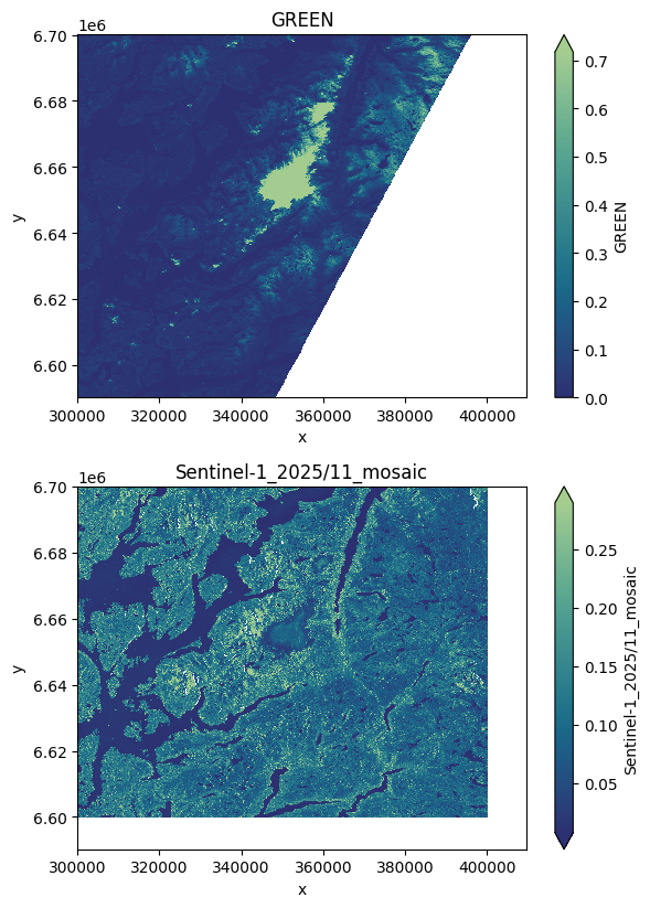
# Plot exogenous bands
ncols = len(loaded_bands)
plt.figure(figsize=(6, 6 * ncols), layout="tight")
i = 0
for key in loaded_bands.keys():
    axes = plt.subplot(3, 1, i+1)
    loaded_bands[key][0, ...].plot.imshow(robust=True, cmap="crest_r")
    axes.set_title(to_str(loaded_bands[key].name)[0])
    i += 1

These arguments can be used the same way to create a stack:

# Stack on an AOI
stack = prod.stack(
  ['RED', 'SWIR_1'],
  pixel_size=100.,
  window=exo_folder / "aoi.shp",
  stack_path=prod.output / "stack_exo.tif",
    **{
        EXO_KW: {'Sentinel-1_2025/11_mosaic': {'path' : mosaic_s1, 'resampler' : Resampling.bilinear}},     
    }
)

2025-12-23 11:44:28,979 - [DEBUG] - Loading bands ['RED', 'SWIR_1']
2025-12-23 11:44:28,990 - [DEBUG] - Read RED
2025-12-23 11:44:29,192 - [DEBUG] - Manage nodata for band RED
2025-12-23 11:44:29,312 - [DEBUG] - Converting RED to reflectance (if needed)
2025-12-23 11:44:29,314 - [DEBUG] - Clip the reflectance array to 0 as minimum value (in some cases, reflectance can have higher value than 1)
2025-12-23 11:44:32,703 - [DEBUG] - Read SWIR_1
2025-12-23 11:44:32,782 - [DEBUG] - Manage nodata for band SWIR_1
2025-12-23 11:44:32,874 - [DEBUG] - Converting SWIR_1 to reflectance (if needed)
2025-12-23 11:44:32,877 - [DEBUG] - Clip the reflectance array to 0 as minimum value (in some cases, reflectance can have higher value than 1)
2025-12-23 11:44:34,839 - [INFO] - Loading exogenous bands
2025-12-23 11:44:34,839 - [DEBUG] - EXO data info: Sentinel-1_2025/11_mosaic ; {'path': PosixPath('/home/prods/EXOGENOUS/Sentinel-1_IW_mosaic_2025_M11_32VLM_0_0_VV.tif'), 'resampler': <Resampling.bilinear: 1>}
2025-12-23 11:44:34,840 - [DEBUG] - Already existing EXO for 20251017T111101_S2_T32VLM_L2A_151300. Skipping process.
2025-12-23 11:44:34,919 - [DEBUG] - Stacking
2025-12-23 11:44:34,941 - [DEBUG] - Saving stack

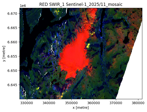
# Plot the stack
(stack / stack.max()).plot.imshow(robust=True)
plt.title(stack.attrs["long_name"]);

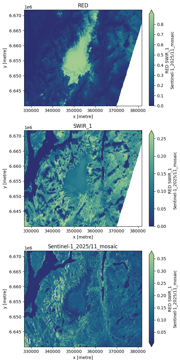
# Plot the stack band per band
ncols = len(stack)
band_names = stack.attrs["long_name"].split(" ")

plt.figure(figsize=(6, 4 * ncols), layout="tight")
for i in range(0, ncols):
    axes = plt.subplot(3, 1, i+1)
    stack[i, ...].plot.imshow(robust=True, cmap="crest_r")
    axes.set_title(band_names[i])
    i += 1