
Optical example
Contents
Optical example#
Let’s use EOReader with optical data.
Imports#
import os
import matplotlib.pyplot as plt

# EOReader
from eoreader.reader import Reader
from eoreader.bands import RED, GREEN, NDVI, YELLOW, CLOUDS, to_str
Open the product#
First, open a Landsat-9 OLI-TIRS collection 2 product.
path = os.path.join("/home", "data", "DATA", "PRODS", "LANDSATS_COL2", "LC09_L1TP_200030_20220201_20220201_02_T1.tar")
reader = Reader()
prod = reader.open(path)
prod
eoreader.LandsatProduct 'LC09_L1TP_200030_20220201_20220201_02_T1'
Attributes:
	condensed_name: 20220201T104852_L9_200030_OLI_TIRS
	path: /home/data/DATA/PRODS/LANDSATS_COL2/LC09_L1TP_200030_20220201_20220201_02_T1.tar
	constellation: Landsat-9
	sensor type: Optical
	product type: L1
	default resolution: 30.0
	acquisition datetime: 2022-02-01T10:48:52
	band mapping:
		COASTAL_AEROSOL: 1
		BLUE: 2
		GREEN: 3
		RED: 4
		NIR: 5
		NARROW_NIR: 5
		CIRRUS: 9
		SWIR_1: 6
		SWIR_2: 7
		THERMAL_IR_1: 10
		THERMAL_IR_2: 11
		PANCHROMATIC: 8
	needs extraction: False
	cloud cover: 49.31
	tile name: 200030
Product information#
You have opened your product, and you have its object in hands.
You can play a little with it to see what it is inside
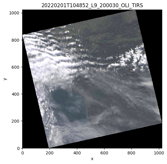
# Plot the quicklook
prod.plot()
/opt/conda/lib/python3.10/site-packages/rasterio/__init__.py:304: NotGeoreferencedWarning: Dataset has no geotransform, gcps, or rpcs. The identity matrix will be returned.
  dataset = DatasetReader(path, driver=driver, sharing=sharing, **kwargs)
/opt/conda/lib/python3.10/site-packages/rioxarray/_io.py:1111: NotGeoreferencedWarning: Dataset has no geotransform, gcps, or rpcs. The identity matrix will be returned.
  warnings.warn(str(rio_warning.message), type(rio_warning.message))  # type: ignore
# Get the band information
prod.bands
eoreader.SpectralBand 'Coastal aerosol'
Attributes:
	id: 1
	eoreader_name: COASTAL_AEROSOL
	common_name: coastal
	gsd (m): 30
	asset_role: reflectance
	Center wavelength (nm): 440.0
	Bandwidth (nm): 20.0
	description: Coastal and aerosol studies
eoreader.SpectralBand 'Blue'
Attributes:
	id: 2
	eoreader_name: BLUE
	common_name: blue
	gsd (m): 30
	asset_role: reflectance
	Center wavelength (nm): 480.0
	Bandwidth (nm): 60.0
	description: Bathymetric mapping, distinguishing soil from vegetation and deciduous from coniferous vegetation
eoreader.SpectralBand 'Green'
Attributes:
	id: 3
	eoreader_name: GREEN
	common_name: green
	gsd (m): 30
	asset_role: reflectance
	Center wavelength (nm): 560.0
	Bandwidth (nm): 60.0
	description: Emphasizes peak vegetation, which is useful for assessing plant vigor
eoreader.SpectralBand 'Red'
Attributes:
	id: 4
	eoreader_name: RED
	common_name: red
	gsd (m): 30
	asset_role: reflectance
	Center wavelength (nm): 655.0
	Bandwidth (nm): 30.0
	description: Discriminates vegetation slopes
eoreader.SpectralBand 'Near Infrared (NIR)'
Attributes:
	id: 5
	eoreader_name: NIR
	common_name: nir
	gsd (m): 30
	asset_role: reflectance
	Center wavelength (nm): 865.0
	Bandwidth (nm): 30.0
	description: Emphasizes biomass content and shorelines
eoreader.SpectralBand 'Near Infrared (NIR)'
Attributes:
	id: 5
	eoreader_name: NARROW_NIR
	common_name: nir08
	gsd (m): 30
	asset_role: reflectance
	Center wavelength (nm): 865.0
	Bandwidth (nm): 30.0
	description: Emphasizes biomass content and shorelines
eoreader.SpectralBand 'SWIR 1'
Attributes:
	id: 6
	eoreader_name: SWIR_1
	common_name: swir16
	gsd (m): 30
	asset_role: reflectance
	Center wavelength (nm): 1610.0
	Bandwidth (nm): 80.0
	description: Discriminates moisture content of soil and vegetation; penetrates thin clouds
eoreader.SpectralBand 'SWIR 2'
Attributes:
	id: 7
	eoreader_name: SWIR_2
	common_name: swir22
	gsd (m): 30
	asset_role: reflectance
	Center wavelength (nm): 2200.0
	Bandwidth (nm): 180.0
	description: Improved moisture content of soil and vegetation; penetrates thin clouds
eoreader.SpectralBand 'Panchromatic'
Attributes:
	id: 8
	eoreader_name: PANCHROMATIC
	common_name: pan
	gsd (m): 30
	asset_role: reflectance
	Center wavelength (nm): 590.0
	Bandwidth (nm): 180.0
	description: 15 meter resolution, sharper image definition
eoreader.SpectralBand 'Cirrus'
Attributes:
	id: 9
	eoreader_name: CIRRUS
	common_name: cirrus
	gsd (m): 30
	asset_role: reflectance
	Center wavelength (nm): 1370.0
	Bandwidth (nm): 20.0
	description: Improved detection of cirrus cloud contamination
eoreader.SpectralBand 'Thermal Infrared (TIRS) 1'
Attributes:
	id: 10
	eoreader_name: THERMAL_IR_1
	common_name: lwir11
	gsd (m): 100
	asset_role: brightness_temperature
	Center wavelength (nm): 10895.0
	Bandwidth (nm): 590.0
	description: 100 meter resolution, thermal mapping and estimated soil moisture
eoreader.SpectralBand 'Thermal Infrared (TIRS) 2'
Attributes:
	id: 11
	eoreader_name: THERMAL_IR_2
	common_name: lwir12
	gsd (m): 100
	asset_role: brightness_temperature
	Center wavelength (nm): 12005.0
	Bandwidth (nm): 1010.0
	description: 100 meter resolution, improved thermal mapping and estimated soil moisture
# Some other information
print(f"Acquisition datetime: {prod.datetime}")
print(f"Condensed name: {prod.condensed_name}")
print(f"Landsat tile: {prod.tile_name}")
Acquisition datetime: 2022-02-01 10:48:52
Condensed name: 20220201T104852_L9_200030_OLI_TIRS
Landsat tile: 200030
# Retrieve the UTM CRS of the tile
prod.crs()
CRS.from_epsg(32630)
# Open here some more interesting geographical data: extent and footprint
extent = prod.extent()
footprint = prod.footprint()

base = extent.plot(color='cyan', edgecolor='black')
footprint.plot(ax=base, color='blue', edgecolor='black', alpha=0.5)
<AxesSubplot: >
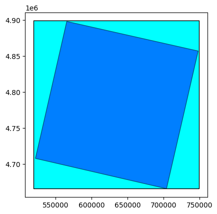
See the difference between footprint and extent hereunder:
Without nodata |
With nodata |
|---|---|
|
|
Load bands#
Let’s open some spectral and cloud bands.
# Select some bands you want to load
bands = [GREEN, NDVI, YELLOW, CLOUDS]

# Be sure they exist for Landsat-9 OLI-TIRS sensor:
ok_bands = [band for band in bands if prod.has_band(band)]
print(to_str(ok_bands))
# Landsat-9 OLI-TIRS doesn't provide YELLOW band
['GREEN', 'NDVI', 'CLOUDS']
# Load those bands as a dict of xarray.DataArray
band_dict = prod.load(ok_bands)
band_dict[GREEN]
<xarray.DataArray 'GREEN' (band: 1, y: 7791, x: 7681)>
array([[[nan, nan, nan, ..., nan, nan, nan],
        [nan, nan, nan, ..., nan, nan, nan],
        [nan, nan, nan, ..., nan, nan, nan],
        ...,
        [nan, nan, nan, ..., nan, nan, nan],
        [nan, nan, nan, ..., nan, nan, nan],
        [nan, nan, nan, ..., nan, nan, nan]]], dtype=float32)
Coordinates:
  * band         (band) int64 1
  * x            (x) float64 5.193e+05 5.193e+05 ... 7.497e+05 7.497e+05
  * y            (y) float64 4.899e+06 4.899e+06 ... 4.665e+06 4.665e+06
    spatial_ref  int64 0
Attributes: (12/13)
    long_name:         GREEN
    constellation:     Landsat-9
    constellation_id:  L9
    product_path:      /home/data/DATA/PRODS/LANDSATS_COL2/LC09_L1TP_200030_2...
    product_name:      LC09_L1TP_200030_20220201_20220201_02_T1
    product_filename:  LC09_L1TP_200030_20220201_20220201_02_T1
    ...                ...
    product_type:      L1
    acquisition_date:  20220201T104852
    condensed_name:    20220201T104852_L9_200030_OLI_TIRS
    orbit_direction:   DESCENDING
    radiometry:        reflectance
cloud_cover: 49.31# The nan corresponds to the nodata you see on the footprint
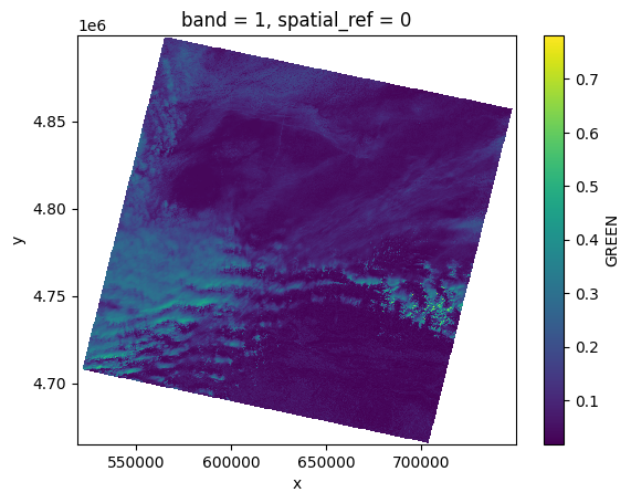
# Plot a subsampled version
band_dict[GREEN][:, ::10, ::10].plot()
<matplotlib.collections.QuadMesh at 0x7fa621f9f190>
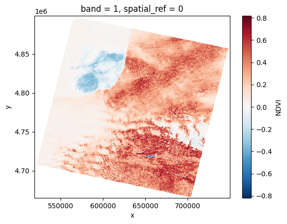
# Plot a subsampled version
band_dict[NDVI][:, ::10, ::10].plot()
<matplotlib.collections.QuadMesh at 0x7fa62235fbe0>
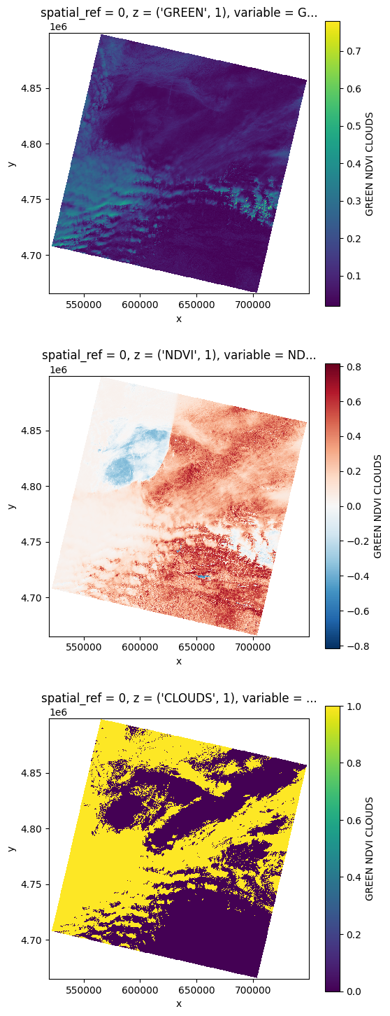
Load a stack#
You can also stack the bands you requested right before
# You can also stack those bands
stack = prod.stack(ok_bands)
stack
<xarray.DataArray 'GREEN_NDVI_CLOUDS' (z: 3, y: 7791, x: 7681)>
array([[[nan, nan, nan, ..., nan, nan, nan],
[nan, nan, nan, ..., nan, nan, nan],
[nan, nan, nan, ..., nan, nan, nan],
...,
[nan, nan, nan, ..., nan, nan, nan],
[nan, nan, nan, ..., nan, nan, nan],
[nan, nan, nan, ..., nan, nan, nan]],
[[nan, nan, nan, ..., nan, nan, nan],
[nan, nan, nan, ..., nan, nan, nan],
[nan, nan, nan, ..., nan, nan, nan],
...,
[nan, nan, nan, ..., nan, nan, nan],
[nan, nan, nan, ..., nan, nan, nan],
[nan, nan, nan, ..., nan, nan, nan]],
[[nan, nan, nan, ..., nan, nan, nan],
[nan, nan, nan, ..., nan, nan, nan],
[nan, nan, nan, ..., nan, nan, nan],
...,
[nan, nan, nan, ..., nan, nan, nan],
[nan, nan, nan, ..., nan, nan, nan],
[nan, nan, nan, ..., nan, nan, nan]]], dtype=float32)
Coordinates:
* x (x) float64 5.193e+05 5.193e+05 ... 7.497e+05 7.497e+05
* y (y) float64 4.899e+06 4.899e+06 ... 4.665e+06 4.665e+06
spatial_ref int64 0
* z (z) object MultiIndex
* variable (z) object 'GREEN' 'NDVI' 'CLOUDS'
* band (z) int64 1 1 1
Attributes:
long_name: GREEN NDVI CLOUDS
constellation: Landsat-9
constellation_id: L9
product_path: /home/data/DATA/PRODS/LANDSATS_COL2/LC09_L1TP_200030_2...
product_name: LC09_L1TP_200030_20220201_20220201_02_T1
product_filename: LC09_L1TP_200030_20220201_20220201_02_T1
instrument: OLI-TIRS
product_type: L1
acquisition_date: 20220201T104852
condensed_name: 20220201T104852_L9_200030_OLI_TIRS
orbit_direction: DESCENDING
cloud_cover: 49.31# Plot a subsampled version
nrows = len(stack)
fig, axes = plt.subplots(nrows=nrows, figsize=(2 * nrows, 6 * nrows), subplot_kw={"box_aspect": 1}) # Square plots
for i in range(nrows):
stack[i, ::10, ::10].plot(x="x", y="y", ax=axes[i])
Radiometric processing#
EOReader allows you to load the band array as provided (either in DN, scaled radiance or reflectance). However, by default, EOReader converts all optical bands in reflectance (except for the thermal bands that are left if brilliance temperature)
The radiometric processing is described in the band’s attribute, either reflectance or as is
# Reflectance band
from eoreader.keywords import TO_REFLECTANCE
prod.load(RED, **{TO_REFLECTANCE: True})
{<SpectralBandNames.RED: 'RED'>: <xarray.DataArray 'RED' (band: 1, y: 7791, x: 7681)>
array([[[nan, nan, nan, ..., nan, nan, nan],
        [nan, nan, nan, ..., nan, nan, nan],
        [nan, nan, nan, ..., nan, nan, nan],
        ...,
        [nan, nan, nan, ..., nan, nan, nan],
        [nan, nan, nan, ..., nan, nan, nan],
        [nan, nan, nan, ..., nan, nan, nan]]], dtype=float32)
Coordinates:
* band (band) int64 1
* x (x) float64 5.193e+05 5.193e+05 ... 7.497e+05 7.497e+05
* y (y) float64 4.899e+06 4.899e+06 ... 4.665e+06 4.665e+06
spatial_ref int64 0
Attributes: (12/13)
long_name: RED
constellation: Landsat-9
constellation_id: L9
product_path: /home/data/DATA/PRODS/LANDSATS_COL2/LC09_L1TP_200030_2...
product_name: LC09_L1TP_200030_20220201_20220201_02_T1
product_filename: LC09_L1TP_200030_20220201_20220201_02_T1
... ...
product_type: L1
acquisition_date: 20220201T104852
condensed_name: 20220201T104852_L9_200030_OLI_TIRS
orbit_direction: DESCENDING
radiometry: reflectance
cloud_cover: 49.31}
# As is band
prod.load(RED, **{TO_REFLECTANCE: False})
{<SpectralBandNames.RED: 'RED'>: <xarray.DataArray 'RED' (band: 1, y: 7791, x: 7681)>
 array([[[nan, nan, nan, ..., nan, nan, nan],
         [nan, nan, nan, ..., nan, nan, nan],
         [nan, nan, nan, ..., nan, nan, nan],
         ...,
         [nan, nan, nan, ..., nan, nan, nan],
         [nan, nan, nan, ..., nan, nan, nan],
         [nan, nan, nan, ..., nan, nan, nan]]], dtype=float32)
 Coordinates:
   * band         (band) int64 1
   * x            (x) float64 5.193e+05 5.193e+05 ... 7.497e+05 7.497e+05
   * y            (y) float64 4.899e+06 4.899e+06 ... 4.665e+06 4.665e+06
     spatial_ref  int64 0
 Attributes: (12/13)
     long_name:         RED
     constellation:     Landsat-9
     constellation_id:  L9
     product_path:      /home/data/DATA/PRODS/LANDSATS_COL2/LC09_L1TP_200030_2...
     product_name:      LC09_L1TP_200030_20220201_20220201_02_T1
     product_filename:  LC09_L1TP_200030_20220201_20220201_02_T1
     ...                ...
     product_type:      L1
     acquisition_date:  20220201T104852
     condensed_name:    20220201T104852_L9_200030_OLI_TIRS
     orbit_direction:   DESCENDING
     radiometry:        as is
     cloud_cover:       49.31}