Sentinel-3
Contents
Sentinel-3
Let’s use EOReader to open and read some Sentinel-3 bands and see the specificities of OLCI and SLSTR sensors.
Note that Sentinel-3 processes have stopped to use SNAP since the 0.8.0 version.
Some minor discrepancies might occur both in the geocoding (especially OLCI) and the reflectance values (SLSTR).
# Imports
import os
from eoreader.reader import Reader
from eoreader.bands import *

import warnings
import rasterio

# Disable georef warnings here as the SAR products are not georeferenced
warnings.filterwarnings("ignore", category=rasterio.errors.NotGeoreferencedWarning)

# Declare the reader (only once)
eoreader = Reader()
# Create logger
import logging

logger = logging.getLogger("eoreader")
logger.setLevel(logging.DEBUG)

# create console handler and set level to debug
ch = logging.StreamHandler()
ch.setLevel(logging.DEBUG)

# create formatter
formatter = logging.Formatter('%(message)s')

# add formatter to ch
ch.setFormatter(formatter)

# add ch to logger
logger.addHandler(ch)
Sentinel-3 OLCI
# First of all, let's focus on Sentinel-3 OLCI data
olci_path = os.path.join("/home", "data", "DATA", "PRODS", "S3",
                         "S3A_OL_1_EFR____20191215T105023_20191215T105323_20191216T153115_0179_052_322_2160_LN1_O_NT_002.zip")
olci_prod = eoreader.open(olci_path, remove_tmp=True)
olci_prod
EOReader S3OlciProduct
Attributes:
	condensed_name: 20191215T105023_S3_OLCI_EFR
	name: S3A_OL_1_EFR____20191215T105023_20191215T105323_20191216T153115_0179_052_322_2160_LN1_O_NT_002
	path: /home/data/DATA/PRODS/S3/S3A_OL_1_EFR____20191215T105023_20191215T105323_20191216T153115_0179_052_322_2160_LN1_O_NT_002.zip
	platform: Sentinel-3 OLCI
	sensor type: Optical
	product type: OL_1_EFR___
	default resolution: 300.0
	acquisition datetime: 2019-12-15T10:50:23.000506
	band mapping:
		COASTAL_AEROSOL: Oa03
		BLUE: Oa04
		GREEN: Oa06
		YELLOW: Oa07
		RED: Oa08
		VEGETATION_RED_EDGE_1: Oa11
		VEGETATION_RED_EDGE_2: Oa12
		VEGETATION_RED_EDGE_3: Oa16
		NIR: Oa17
		NARROW_NIR: Oa17
		WATER_VAPOUR: Oa20
		Oa01: Oa01
		Oa02: Oa02
		Oa05: Oa05
		Oa09: Oa09
		Oa10: Oa10
		Oa13: Oa13
		Oa14: Oa14
		Oa15: Oa15
		Oa18: Oa18
		Oa19: Oa19
		Oa21: Oa21
	tile name: N/A
	needs_extraction: False
# Load the Yellow band and the far NIR one
# Please note that mapped band need to be called by their mapped name and the specific one with their true name
olci_bands = olci_prod.load([YELLOW, Oa21])
Loading bands ['YELLOW', 'Oa21']
Converting YELLOW to reflectance
Geocoding YELLOW
Converting Oa21 to reflectance
Geocoding Oa21
Read YELLOW
Manage nodata for band YELLOW
Read Oa21
Manage nodata for band Oa21
# Plot a subsampled version
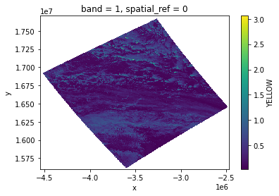
olci_bands[YELLOW][:, ::10, ::10].plot()
<matplotlib.collections.QuadMesh at 0x7fec2c31a340>
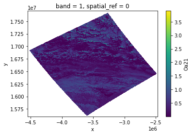
olci_bands[Oa21][:, ::10, ::10].plot()
<matplotlib.collections.QuadMesh at 0x7fec2c192790>
Sentinel-3 SLSTR
# Other imports
from eoreader.keywords import SLSTR_VIEW, SLSTR_STRIPE, SLSTR_RAD_ADJUST
from eoreader.products import SlstrRadAdjustTuple, SlstrRadAdjust, SlstrView, SlstrStripe

# Then, let's focus on Sentinel-3 SLSTR data (extracted here, but a zip would work)
slstr_path = os.path.join("/home", "data", "DATA", "PRODS", "S3",
                          "S3B_SL_1_RBT____20191115T233722_20191115T234022_20191117T031722_0179_032_144_3420_LN2_O_NT_003.SEN3")
slstr_prod = eoreader.open(slstr_path, remove_tmp=True)
slstr_prod
EOReader S3SlstrProduct
Attributes:
	condensed_name: 20191115T233722_S3_SLSTR_RBT
	name: S3B_SL_1_RBT____20191115T233722_20191115T234022_20191117T031722_0179_032_144_3420_LN2_O_NT_003
	path: /home/data/DATA/PRODS/S3/S3B_SL_1_RBT____20191115T233722_20191115T234022_20191117T031722_0179_032_144_3420_LN2_O_NT_003.SEN3
	platform: Sentinel-3 SLSTR
	sensor type: Optical
	product type: SL_1_RBT___
	default resolution: 500.0
	acquisition datetime: 2019-11-15T23:37:22.254773
	band mapping:
		GREEN: S1
		RED: S2
		NIR: S3
		NARROW_NIR: S3
		CIRRUS: S4
		SWIR_1: S5
		SWIR_2: S6
		THERMAL_IR_1: S8
		THERMAL_IR_2: S9
		S7: S7
		F1: F1
		F2: F2
	tile name: N/A
	needs_extraction: True
# Same remark for mapped and specific band than above
# Not that native radiance band are converted into reflectance, whereas brilliance temperature bands are not
# Load bands with nadir view and stripe B
# (for bands that have a stripe B, the other will load their unique stripe, namely A or I)
# RED: only stripe A
# SWIR_2: has strip 1, B and TDI (c)
# F1: has only stripe I
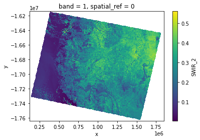
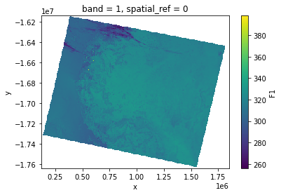
slstr_bn_bands = slstr_prod.load([RED, SWIR_2, F1], slstr_view="n", slstr_stripe="b")
slstr_bn_bands_2 = slstr_prod.load([RED, SWIR_2, F1], **{SLSTR_VIEW: SlstrView.NADIR, SLSTR_STRIPE: SlstrStripe.B})
Loading bands ['SWIR_2', 'RED', 'F1']
Converting SWIR_2 to reflectance
Geocoding SWIR_2
Converting RED to reflectance
Geocoding RED
Geocoding F1
Read SWIR_2
Manage nodata for band SWIR_2
Read RED
Manage nodata for band RED
Read F1
Manage nodata for band F1
Loading bands ['SWIR_2', 'RED', 'F1']
Read SWIR_2
Read RED
Read F1
# You can use the keywords by importing them or copy their value.
# Their values can be passed as strings or as an Enum
# However, it seems safer to import the keywords and use the enum
# The result should be the same

# Please bear in mind that oblique and nadir views are not stackable !
# However, you can stack different stripes
# (but you cannot load them at once and you should collocate them to be sure, their reprojection grid may vary as their GCP vary)
# Plot a subsampled version
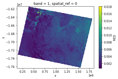
slstr_bn_bands[RED][:, ::10, ::10].plot()
<matplotlib.collections.QuadMesh at 0x7fec2b6ed700>
slstr_bn_bands[SWIR_2][:, ::10, ::10].plot()
<matplotlib.collections.QuadMesh at 0x7fec2b6a3a90>
slstr_bn_bands[F1][:, ::10, ::10].plot()
<matplotlib.collections.QuadMesh at 0x7fec2b59c4f0>
# Sentinel-3 SLSTR radiance is not nominal, so EUMETSAT advises the user to make some radiance adjustments
# As stated here: https://www-cdn.eumetsat.int/files/2021-05/S3.PN-SLSTR-L1.08%20-%20i1r0%20-%20SLSTR%20L1%20PB%202.75-A%20and%201.53-B.pdf
# These coefficients have been added since the 06 version and several sets exist:

# The last one (S3.PN-SLSTR-L1.08, since 18/05/2021) which is also the default one
SlstrRadAdjust.S3_PN_SLSTR_L1_08
<SlstrRadAdjust.S3_PN_SLSTR_L1_08: SlstrRadAdjustTuple(S1_n=0.97, S2_n=0.98, S3_n=0.98, S4_n=1.0, S5_n=1.11, S6_n=1.13, S1_o=0.94, S2_o=0.95, S3_o=0.95, S4_o=1.0, S5_o=1.04, S6_o=1.07)>
# The two older sets given by EUMETSAT are the same
assert SlstrRadAdjust.S3_PN_SLSTR_L1_07 == SlstrRadAdjust.S3_PN_SLSTR_L1_06
SlstrRadAdjust.S3_PN_SLSTR_L1_07
<SlstrRadAdjust.S3_PN_SLSTR_L1_06: SlstrRadAdjustTuple(S1_n=1.0, S2_n=1.0, S3_n=1.0, S4_n=1.0, S5_n=1.12, S6_n=1.15, S1_o=1.0, S2_o=1.0, S3_o=1.0, S4_o=1.0, S5_o=1.2, S6_o=1.26)>
# Moreover, SNAP uses a different set with unknown origin (optional, in S3MPC Calibration)
SlstrRadAdjust.SNAP
<SlstrRadAdjust.SNAP: SlstrRadAdjustTuple(S1_n=1.0, S2_n=1.0, S3_n=1.0, S4_n=1.0, S5_n=1.12, S6_n=1.13, S1_o=1.0, S2_o=1.0, S3_o=1.0, S4_o=1.0, S5_o=1.15, S6_o=1.14)>
# A default set also exists, with every coefficient set to 1.0
SlstrRadAdjust.NONE
<SlstrRadAdjust.NONE: SlstrRadAdjustTuple(S1_n=1.0, S2_n=1.0, S3_n=1.0, S4_n=1.0, S5_n=1.0, S6_n=1.0, S1_o=1.0, S2_o=1.0, S3_o=1.0, S4_o=1.0, S5_o=1.0, S6_o=1.0)>
# You can use your own set by creating one.
# All the coefficients are set to 1.0 by default, so just modify the one you want
# The band keywords are {true_name}_{view_letter}
# RED is S2
user_set = SlstrRadAdjustTuple(S1_n=1.15, S2_o=1.12)
# However please bear in mind that if you want to reload the same band with a different adjustment,
# you have to remove the temporary process folder or the previous band will be reloaded.
slstr_prod.clean_tmp()
# To apply these sets when loading a band, just add the keyword when loading it
red_pn_08 = slstr_bn_bands[RED]
slstr_red_bn = slstr_prod.load(
RED,
**{
SLSTR_VIEW: SlstrView.NADIR,
SLSTR_STRIPE: SlstrStripe.B,
SLSTR_RAD_ADJUST: user_set
}
)
red_user = slstr_red_bn[RED]
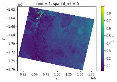
red_user[:, ::10, ::10].plot()
Loading bands ['RED']
Converting RED to reflectance
Geocoding RED
Read RED
Manage nodata for band RED
<matplotlib.collections.QuadMesh at 0x7fec2b2bebe0>

# We may need to collocate the bands if we want to work on two sets loaded apart
# Indeed, in EOReader, the bands are collocated when loaded together

# For example, if we wanted to work on the SWIR or F1 band,
# as we first loaded them with the RED, they are collocated to this band (the first one)
# Yet, their geodetic grid are different from the RED one (in and bn are slightly different than the an)
# So if we load on a second time only the SWIR or the F1 band, their are chances that the geocoding might be a little different
# The it is best to collocate the two bands just to be sure they will always match (and have the same size)

# To do so you could do:
from sertit import rasters

red_user = rasters.collocate(master_xds=red_pn_08, slave_xds=red_user)

# Here, it is useless as we work on the master band
abs(red_pn_08 - red_user)[:, ::10, ::10].plot()
<matplotlib.collections.QuadMesh at 0x7fec2b444a00>