VHR example
VHR example
Let’s use EOReader with Very High Resolution data.
import os
import glob

# First of all, we need some VHR data, let's use Pleiades data
path = glob.glob(os.path.join("/home", "data", "DATA", "PRODS", "PLEIADES", "5547047101", "IMG_PHR1A_PMS_001"))[0]
# Create logger
import logging

logger = logging.getLogger("eoreader")
logger.setLevel(logging.INFO)

# create console handler and set level to debug
ch = logging.StreamHandler()
ch.setLevel(logging.INFO)

# create formatter
formatter = logging.Formatter('%(message)s')

# add formatter to ch
ch.setFormatter(formatter)

# add ch to logger
logger.addHandler(ch)
from eoreader.reader import Reader

# Create the reader
eoreader = Reader()
# Open your product
prod = eoreader.open(path, remove_tmp=True)
print(f"Acquisition datetime: {prod.datetime}")
print(f"Condensed name: {prod.condensed_name}")

# Please be aware that EOReader will always work in UTM projection, so if you give WGS84 data,
# EOReader will reproject the stacks and this can be time consuming
Acquisition datetime: 2020-05-11 02:31:58
Condensed name: 20200511T023158_PLD_ORT_PMS
from eoreader.bands import *
from eoreader.env_vars import DEM_PATH

# Here, if you want to orthorectify or pansharpen your data manually, you can set your stack here.
# If you do not provide this stack but you give a non-orthorectified product to EOReader
# (ie. SEN or PRJ products for Pleiades), you must provide a DEM to orthorectify correctly the data
# prod.ortho_stack = ""
os.environ[DEM_PATH] = os.path.join("/home", "data", "DS2", "BASES_DE_DONNEES", "GLOBAL",
                                    "MERIT_Hydrologically_Adjusted_Elevations", "MERIT_DEM.vrt")
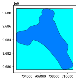
# Open here some more interesting geographical data: extent and footprint
base = prod.extent.plot(color='cyan', edgecolor='black')
prod.footprint.plot(ax=base, color='blue', edgecolor='black', alpha=0.5)
<AxesSubplot:>
# Select the bands you want to load
bands = [GREEN, NDVI, TIR_1, CLOUDS, HILLSHADE]

# Be sure they exist for Pleiades sensor:
ok_bands = [band for band in bands if prod.has_band(band)]
print(to_str(ok_bands))  # Pleiades doesn't provide TIR and SHADOWS bands
['GREEN', 'NDVI', 'CLOUDS', 'HILLSHADE']
# Load those bands as a dict of xarray.DataArray
band_dict = prod.load(ok_bands)
band_dict[GREEN]
Reprojecting band NIR to UTM with a 0.5 m resolution.
Reprojecting band RED to UTM with a 0.5 m resolution.
Reprojecting band GREEN to UTM with a 0.5 m resolution.
<xarray.DataArray 'GREEN' (band: 1, y: 18124, x: 16754)>
array([[[nan, nan, nan, ..., nan, nan, nan],
        [nan, nan, nan, ..., nan, nan, nan],
        [nan, nan, nan, ..., nan, nan, nan],
        ...,
        [nan, nan, nan, ..., nan, nan, nan],
        [nan, nan, nan, ..., nan, nan, nan],
        [nan, nan, nan, ..., nan, nan, nan]]], dtype=float32)
Coordinates:
  * band         (band) int64 1
  * x            (x) float64 7.024e+05 7.024e+05 ... 7.108e+05 7.108e+05
  * y            (y) float64 9.689e+06 9.689e+06 9.689e+06 ... 9.68e+06 9.68e+06
    spatial_ref  int64 0
Attributes:
    scale_factor:      1.0
    add_offset:        0.0
    long_name:         GREEN
    sensor:            Pleiades
    sensor_id:         PLD
    product_path:      /home/data/DATA/PRODS/PLEIADES/5547047101/IMG_PHR1A_PM...
    product_name:      PHR1A_PMS_202005110231585_ORT_5547047101
    product_filename:  IMG_PHR1A_PMS_001
    product_type:      Ortho Single Image
    acquisition_date:  20200511T023158
condensed_name: 20200511T023158_PLD_ORT_PMS# The nan corresponds to the nodata you see on the footprint
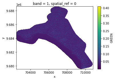
# Plot a subsampled version
band_dict[GREEN][:, ::10, ::10].plot()
<matplotlib.collections.QuadMesh at 0x7f4370284460>
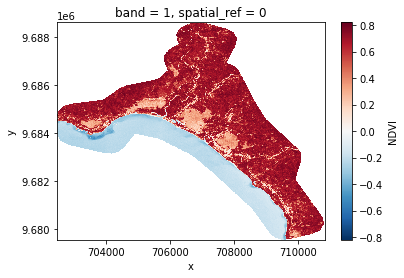
# Plot a subsampled version
band_dict[NDVI][:, ::10, ::10].plot()
<matplotlib.collections.QuadMesh at 0x7f43701973a0>
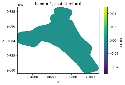
# Plot a subsampled version
band_dict[CLOUDS][:, ::10, ::10].plot()
<matplotlib.collections.QuadMesh at 0x7f43702bd9a0>
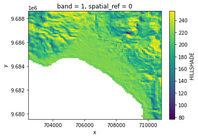
# Plot a subsampled version
band_dict[HILLSHADE][:, ::10, ::10].plot()
<matplotlib.collections.QuadMesh at 0x7f437010fbb0>
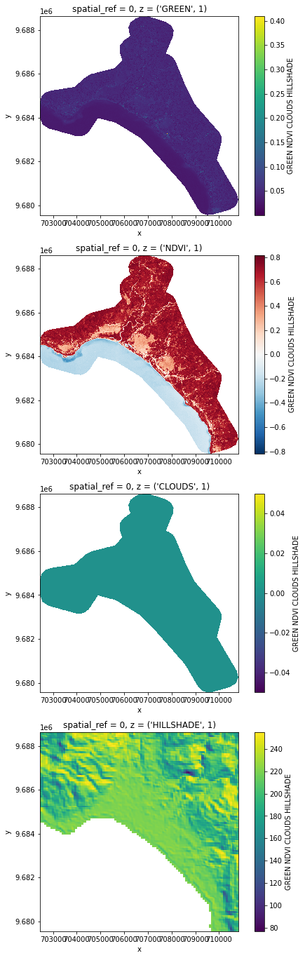
# You can also stack those bands
stack = prod.stack(ok_bands)
stack
<xarray.DataArray 'GREEN NDVI CLOUDS HILLSHADE' (z: 4, y: 18124, x: 16754)>
array([[[      nan,       nan,       nan, ...,       nan,       nan,
               nan],
        [      nan,       nan,       nan, ...,       nan,       nan,
               nan],
        [      nan,       nan,       nan, ...,       nan,       nan,
               nan],
        ...,
        [      nan,       nan,       nan, ...,       nan,       nan,
               nan],
        [      nan,       nan,       nan, ...,       nan,       nan,
               nan],
        [      nan,       nan,       nan, ...,       nan,       nan,
               nan]],

       [[      nan,       nan,       nan, ...,       nan,       nan,
               nan],
        [      nan,       nan,       nan, ...,       nan,       nan,
               nan],
        [      nan,       nan,       nan, ...,       nan,       nan,
               nan],
...
        [      nan,       nan,       nan, ...,       nan,       nan,
               nan],
        [      nan,       nan,       nan, ...,       nan,       nan,
               nan],
        [      nan,       nan,       nan, ...,       nan,       nan,
               nan]],

       [[203.14804, 203.09644, 203.04478, ..., 192.94646, 193.02295,
         193.11148],
        [203.2448 , 203.1972 , 203.14554, ..., 192.77391, 192.85446,
         192.9325 ],
        [203.34145, 203.29594, 203.25027, ..., 192.6033 , 192.6816 ,
         192.76187],
        ...,
        [      nan,       nan,       nan, ..., 174.02263, 173.97194,
         173.9212 ],
        [      nan,       nan,       nan, ..., 176.22513, 176.15732,
         176.08734],
        [      nan,       nan,       nan, ..., 177.34239, 177.27248,
         177.19945]]], dtype=float32)
Coordinates:
    spatial_ref  int64 0
  * x            (x) float64 7.024e+05 7.024e+05 ... 7.108e+05 7.108e+05
  * y            (y) float64 9.689e+06 9.689e+06 9.689e+06 ... 9.68e+06 9.68e+06
  * z            (z) MultiIndex
  - variable     (z) object 'GREEN' 'NDVI' 'CLOUDS' 'HILLSHADE'
  - band         (z) int64 1 1 1 1
Attributes:
    long_name:         GREEN NDVI CLOUDS HILLSHADE
    sensor:            Pleiades
    sensor_id:         PLD
    product_path:      /home/data/DATA/PRODS/PLEIADES/5547047101/IMG_PHR1A_PM...
    product_name:      PHR1A_PMS_202005110231585_ORT_5547047101
    product_filename:  IMG_PHR1A_PMS_001
    product_type:      Ortho Single Image
    acquisition_date:  20200511T023158
condensed_name: 20200511T023158_PLD_ORT_PMS# Plot a subsampled version
import matplotlib.pyplot as plt
nrows = len(stack)
fig, axes = plt.subplots(nrows=nrows, figsize=(2 * nrows, 6 * nrows), subplot_kw={"box_aspect": 1})
for i in range(nrows):
stack[i, ::10, ::10].plot(x="x", y="y", ax=axes[i])